The Impulse Response module for AudioTools or standalone application provides an easy way to capture an IR audio file on iOS devices, and also calculates the most-needed metrics from the data. Impulse Response is an iOS port of a powerful mathematical model developed on desktop computers by Daniel Valente, Ph.D Architectural Acoustics, Rensselaer Polytechnic Institute. In seconds, a complete set of measurements is made that describe the acoustic character of a room, or the response of a loudspeaker.
Impulse Response on the iOS device will give you very good results, even with the built-in mic. Of course, you are limited to moderate SPL levels, and the lowest frequency bands will not be as accurate as when used with iAudioInterface2 or iTestMic, but Impulse Response will give you accurate reverb decay times and other measurements.

Available in AudioTools on the App Store
When you first access the Impulse Response recording screen, the reference chirp files will be downloaded. Or, you install them directly using iTunes. This is especially useful if you are using the Surround Signal Generator.
Be sure to check out our Impulse Response demo videos. Also see our two new videos, New Features in Impulse Response, and Gated Loudspeaker Measurements.
The Impulse Response can be computed either from recording an actual impulse, like a balloon pop or handclap, or from recording a swept sine wave chirp file which is the converted to an impulse through deconvolution, all from within the iPhone.
Important: make sure you download our IR chirp files below, and play them from another iPod or a CD when recording an impulse response chirp, or play them from the iOS device. If you have not downloaded them in a while, please update to the latest versions on this page for best results.
Recording an Impulse Response
You can record either an actual impulse, or a swept sine wave that the app will deconvolve into an impulse. If you plan on recording a swept sine wave chirp file, download our three excitation signal files and burn them to a CD or put them on another iPod.
You can also play the chirps on another iOS device with Remote Control Generator. Also, you can use AudioTools Wireless for remote recording of Impulse Response files.
See our demo video on recording an impulse response.
To record your impulse response, go to the Impulse Response module in AudioTools, and tap the sine wave icon, which will bring up the Recording screen. The first time that you access this screen, the three reference swept sine chirp signal files will be downloaded from our server and saved on your device. You can always re-download them by tapping the “reload” button. This could become necessary if we change the chirp files in the future.
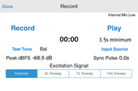
Next, select the type of impulse response that you will be recording: Impulse, 3 second chirp 7 second chirp or 14 second chirp.
Recording an Impulse
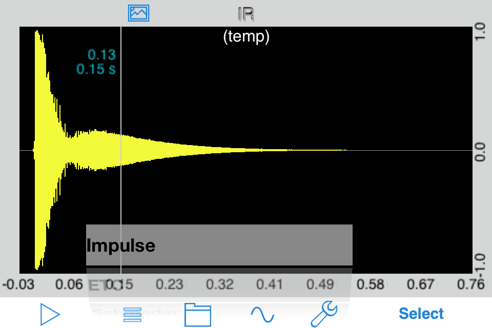
To record an impulse, such as a handclap or balloon pop, just start recording, and create the impulse. Make sure that the Clip indicator does not appear. You can also listen to the impulse to check it, by pressing the Play button. When you are happy with the recorded impulse, tap Done to return to the calculations screen.
After recording the impulse, tap Done to get back to the main screen, where you will see the ETC of the impulse.
Recording a Swept Sine Wave Chirp File
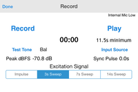
You can select a 3 second, 7 second, or 14 second chirp The tradeoff is that the shorter files process much more quickly, and require less device memory (although we have not yet found a situation where any device has actually run out of memory), and the longer files generally will give you better a better signal to noise ratio (S/N). You may want to start with a 3-second chirp as you get your setup working properly, and then switch to a longer file if you need to.
Next, setup your playback system with the CD or iPod playlist that you created earlier. Connect to a system with only one speaker active, and try playing the sweep. Listen for obvious distortion or other problems.
When you are ready to start recording, tap the Record button on the Recording screen, and then start the chirp playing. You will hear a short sync tone, followed 5 seconds later by the chirp Wait until the minimum time displayed on the screen is reached before tapping Stop to end the recording. Watch the level meter as the chirp runs.
Check that “Clip” does not appear on the screen, and that the chirp got more than half-way up the level meter. The yellow area is perfectly fine. If you like, you can play back the chirp and listen to it.
At the end of the recording, a message box will appear asking whether you want to Deconvolve the chirp or Cancel. If you are happy with the recording, choose Deconvolve. A series of calculations will begin, that make take up to several minutes, depending on the speed of your device. The new models are much faster.
If all goes well, you will see the word “Done” in green, and you can tap Done and go on to the calculations screen. If there is a problem, it will be shown on the screen. The most likely problem is that the sync pulse may not be found. The sync pulse must occur at least one second after starting the recording, and must be within 20dB of the loudest part of the chirp. Also, the recording must be long enough to include at least 5 seconds of decay after the chirp.
When you go back to the calculations screen, the ETC will be computed and shown on the screen. From here you can look at other parameters and metrics, or trim (edit) the IR.
Importing a WAV File
To import a WAV file that was recorded by another device, first copy it to the “import” folder on your iOS device. There are different methods depending on your file storage choice.
The file must be a mono, 16-bit 48kHz wave file.
Internal – If you store files locally on your iOS device, open the iOS Files app, start with On My iPhone or On My iPad, locate the studiosixdigital folder, navigate to the public folder, and then import. This will be the the studiosixdigital/public/import folder. Drag and drop our IR audio wave file into this folder.
iCloud – If you are using iCloud, follow the instructions above, but start with the iCloud Drive folder in the Files app. Now just drag and drop the file into the studiosixdigital/public/import folder .
Once the file is in the import folder, open Impulse Response, and go to the settings page. Scroll down and tap the Import IR button.
Next, go to the Save/Recall page for Impulse Response, and locate the file that you have just imported. If the file contains a valid IR, the results will be shown on the screen. Select the file, and Recall it.
Note that if your file name contains blanks, the name will be altered to replace the blanks.
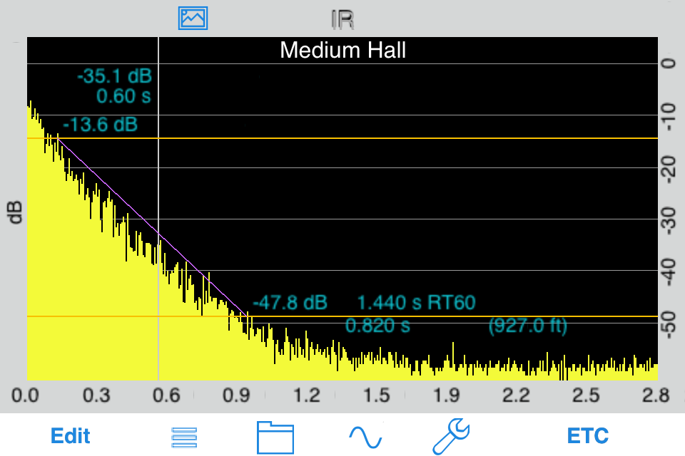
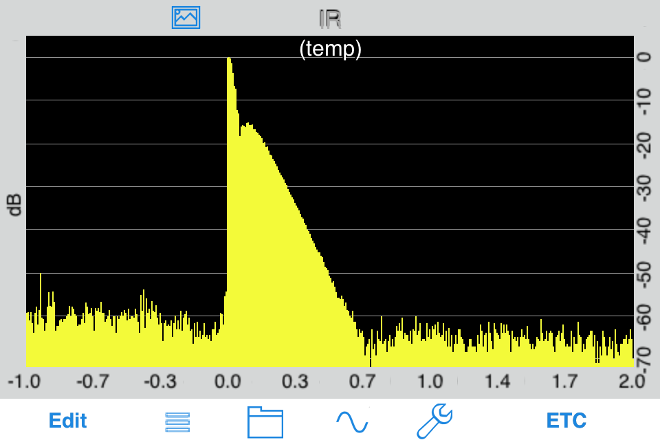
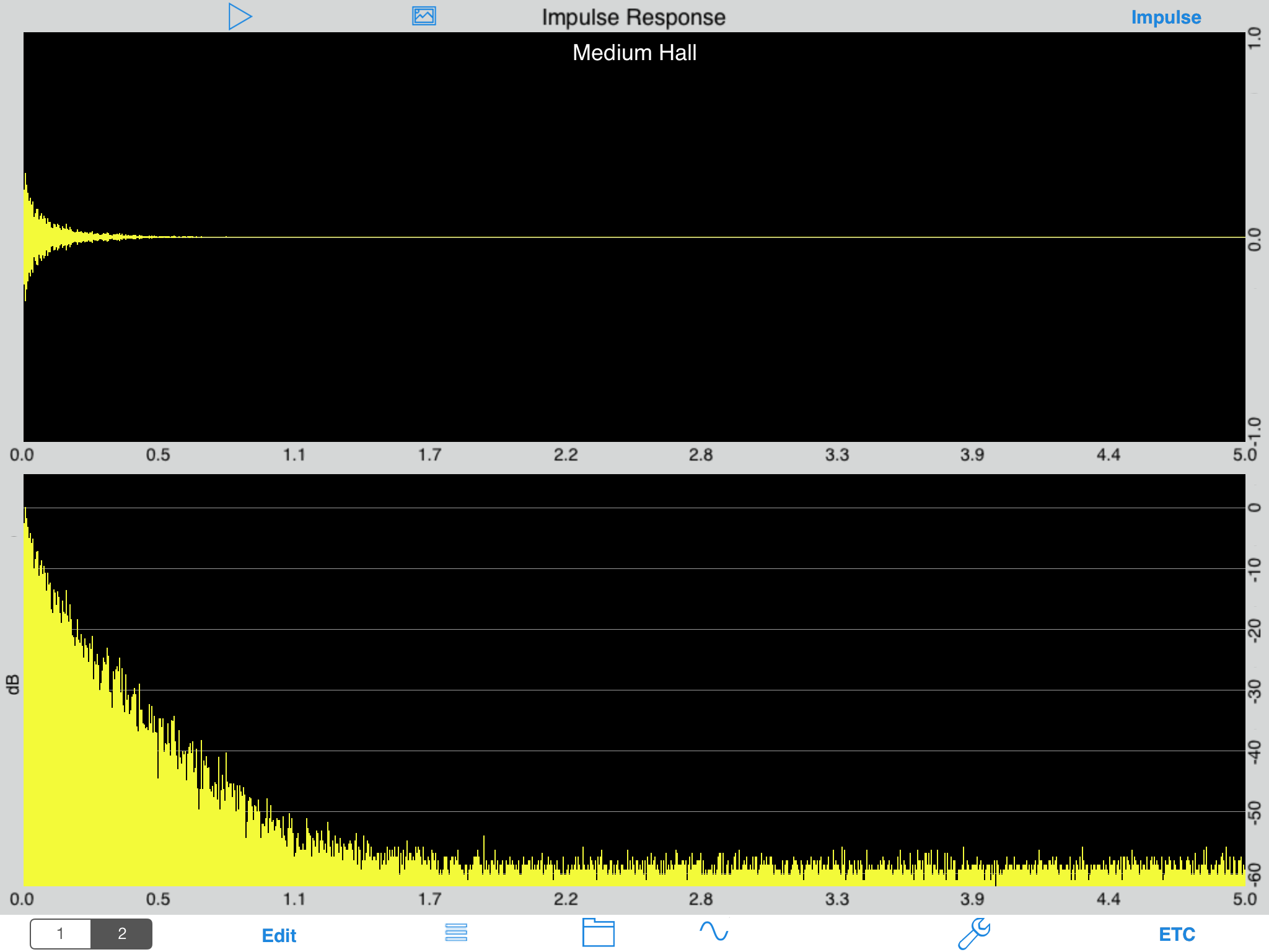
Impulse Plot
 4545
4545The Impulse plot shows the decay of the IR visually. You can use the cursor to read out the exact level magnitude and time.
Also, you can tap the Play button to play the impulse. This can be useful to listen to the sound of a pulse decaying in the room, especially if you have created the impulse from a swept sine, by deconvolution.
You can also use a pinch-zoom gesture to expand the image on the screen to see more detail.
Editing the Impulse Response
Often you can get better results by trimming the start and end of an impulse response. If you have recorded an actual impulse, it is highly recommended that you trim the result. If you have recorded a swept sine, sometimes the resulting IR will need some trimming before the impulse, and the noise after the decay curve can be trimmed to shorten the screen window for a better look at the data.
Before editing IR
When running a swept sine, if the sample rate of the playback device is slightly different than the sample rate of the device that the app is running on, even by just a few Hz, you may see a shorter false peak before the actual impulse. It is important to trim this for the best results.
To edit an IR, go to the ETC screen, and use the pinch/zoom gesture to expand the display. Your goal is to remove extraneous sound before the actual impulse begins, without cutting into the impulse itself, and to remove noise after the decay ends, without cutting into the decay curve itself. The result needs to be at least 0.5 seconds long. 1.0 second is fine.
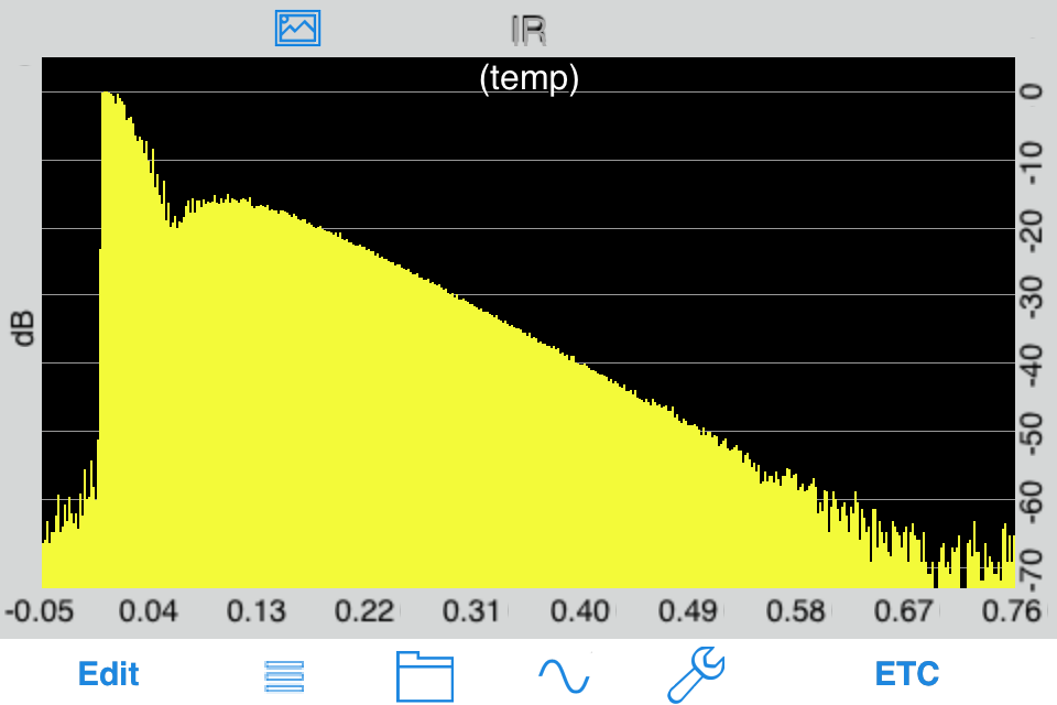
After editing IR
When you have trimmed the ETC, tap the Edit button and select Save File. This will remove the areas of the IR that are not on the screen and the ETC and cause calculations to be re-done.
After trimming, you can then select one of these calculations to display in a bar chart, either by octave band or 1/3 octave band. Calculations are done as needed when you change graph selections.
Windowing the IR
In some cases you will get better calculation results by windowing the IR. Windowing can also be used to inspect a portion of the IR, and to remove reflections from the IR so that you can see the frequency response of a loudspeaker, without the effects of the room. The window is applied before all of the calculations are done, but is used most often in conjunction with the FFT plot, in order to inspect the frequency spectrum of a portion of the IR.
Windowing is controlled by these parameters, which are accessed on the Setup page. Tap the wrench icon to bring up the Setup page.
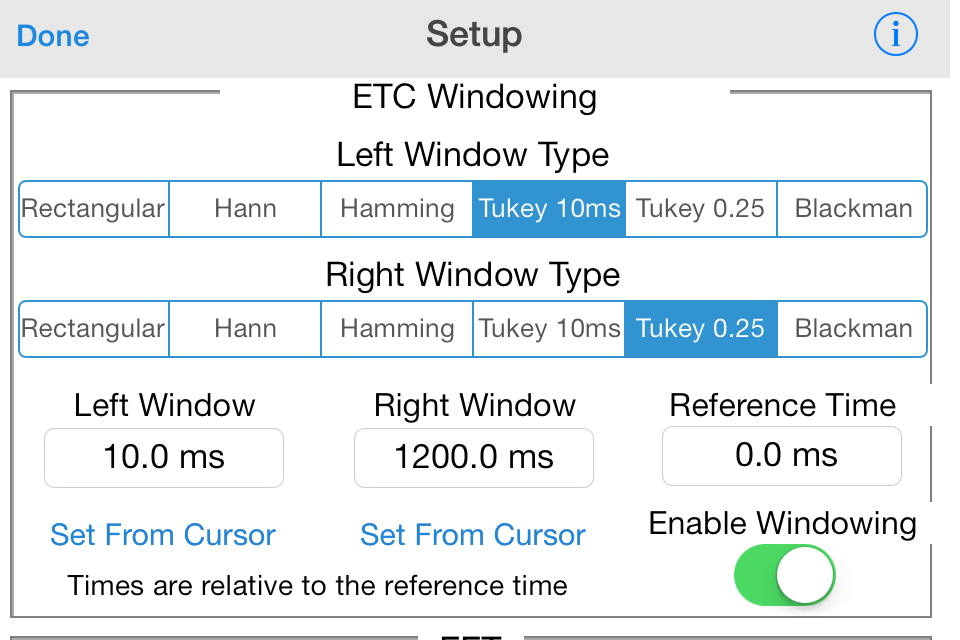
The left and right portions of the window are controlled separately, so that you can precisely control the window.
There are controls here for the size of the left and right windows, and the reference time. Normally you will reference the window to 0.0 ms, which is the time of the peak of the IR. You may shift the windows if you wish to inspect the frequency spectrum at some point in the decay, for example to see the sonic coloring of the room as the signal decays.
You can also select the function that shapes each window. Rectangular is a hard cut of all data before or after the window, but normally you will get a smoother FFT.
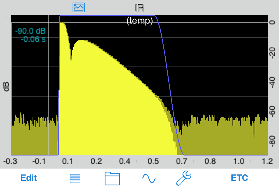
Here is an example of a typical windowed IR, using the settings shown above.
Note that we have windowed out the noise before the direct sound, and we have also windowed out most of the noise after the decay.
This is a typical use of windowing to get better overall IR results. Windowing can also be used to inspect loudspeaker frequency response, independent of room effects.
Octave and 1/3 Octave Bar Charts
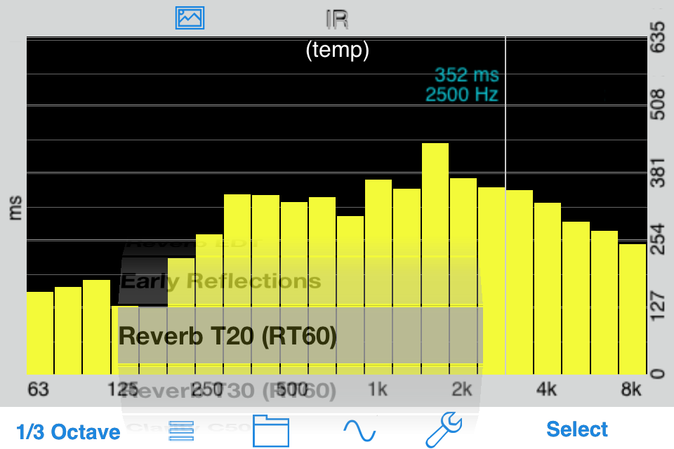
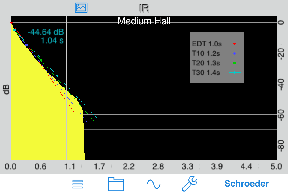
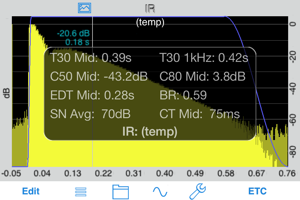
T20 — T20 is the decay rate of the impulse response or reverberation time, the time that is takes for a sound to decay by 60 dB in a space. By using a noise compensation technique to avoid inaccurate representations of reverberation time, the decay rate is calculated by determining the slope of the decay function from -5 dB to -25 dB, and extrapolating the time to a decay of 60 dB.
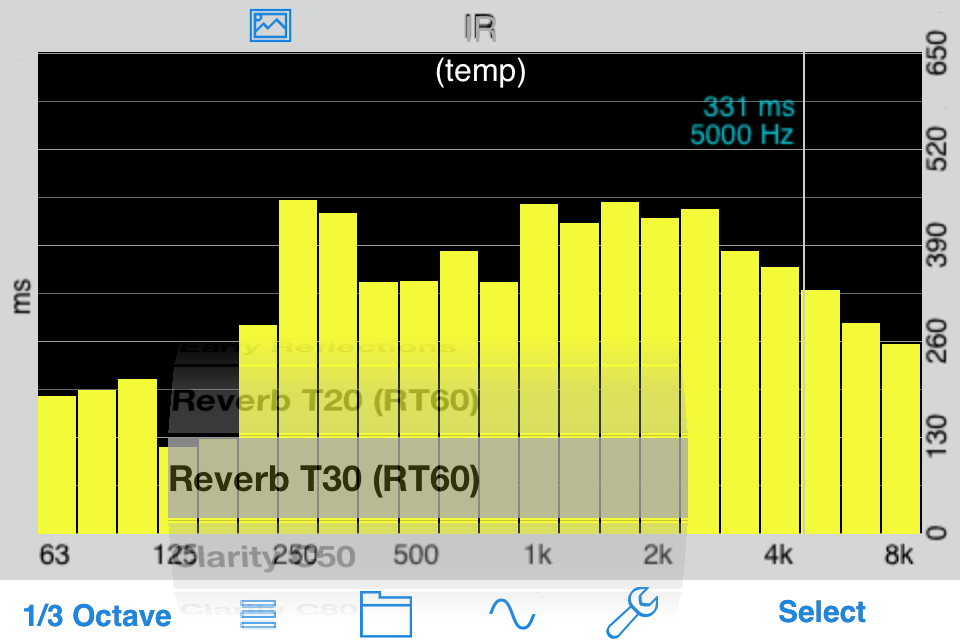
T30 — T30 is the decay rate of the impulse response or reverberation time, the time that is takes for a sound to decay by 60 dB in a space. By using a noise compensation technique to avoid inaccurate representations of reverberation time, the decay rate is calculated by determining the slope of the decay function from -5 dB to -35 dB, and extrapolating the time to a decay of 60 dB.
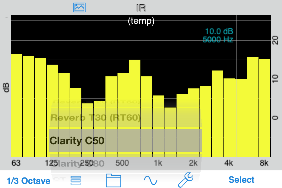
C50 – The Clarity Factor (50ms), expressed in decibels, is the ratio of the early energy (0-50 ms) to the late reverberant energy (50-end of the decay of the IR). C50 is perceptually aligned with speech perception.
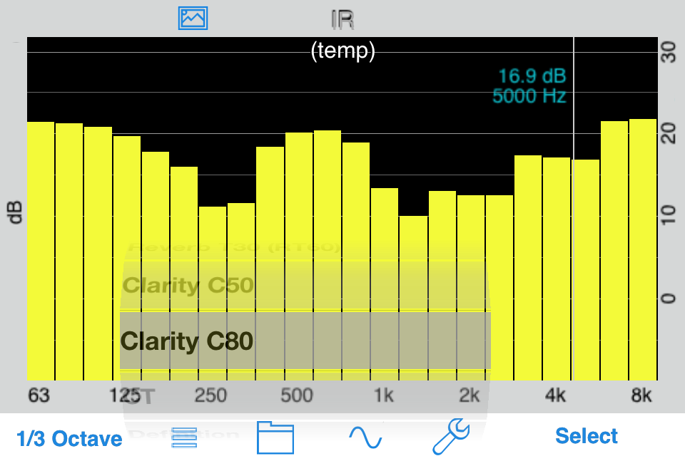
C80 – The Clarity Factor (80ms), expressed in decibels, is the ratio of the early energy (0-80 ms) to the late reverberant energy (80-end of the decay of the IR). C80 is perceptually aligned with music perception.
EDT – Early decay time represents the decay function of the IR in the slope of the early part of the energy decay curve. It is the slope of the curve limited from 0 dB to -10 dB extracted to a decay of 60 dB below to stopping of the direct sound energy. EDT is typically associated with the perceived reverberation time in a room.
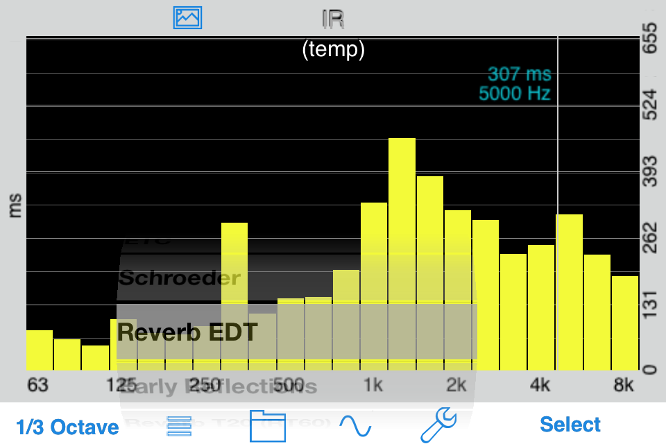
CT – Center time or Ts is the time after the onset of the direct sound to the time where half of the energy has decayed in the IR. It is the time corresponding to the “balancing point” or center of gravity of the squared IR. Center time is correlated with reverberation time, so center time increases as a function of reverberation time.
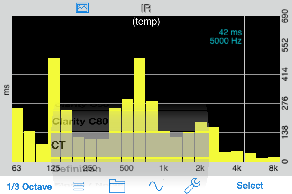
Definition – Similar to the C50 metric, definition represents the ratio of sound arriving in the first 50 ms of the IR compared to the rest of the IR. It is expressed as a percentage and correlates to speech perception in a room
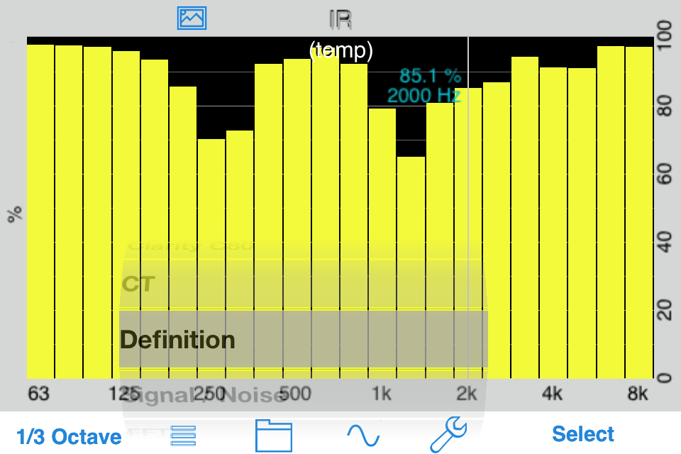
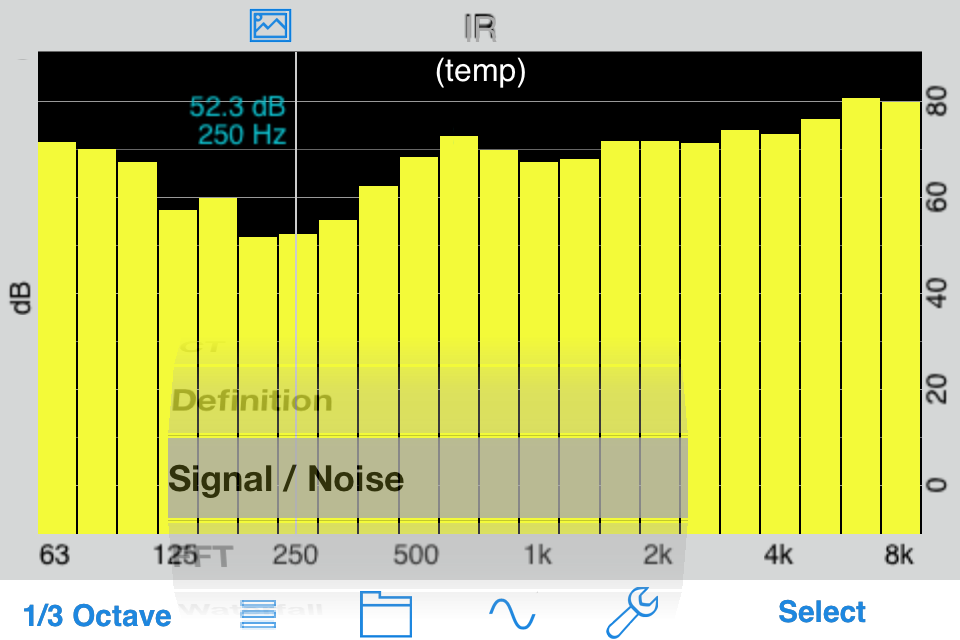
S / N – Signal-to-Noise ratio represents the difference between the measured signal captured by Impulse Response versus the noise floor present in the room under test. It is a good tool to verify that the measurement signal that is being used will yield quality results. Aim for a S/N ratio above 50 dB whenever possible or the reliability of the derived metrics of the IR will be reduced.
Wide-Band Plots
Also, these plots are available, for the wide-band signal:
Schroeder Plot – The backwards integration of the decay function of the impulse response.
ETC — This is the time-domain plot of the decay response of the IR
FFT — The FFT of the ETC results in the frequency response graph for the signal.
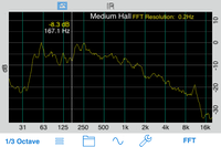
The FFT has a cursor, that you can use to read out the exact dB level and frequency. You may change the smoothing from none to 1/12th, 1/6th, 1/3rd, or octave.
You can also use a pinch-zoom gesture to change either the dB or frequency range. Double-tap to return to full range. Two FFT plots may be seen, and a composite FFT plot may also be derived and drawn.
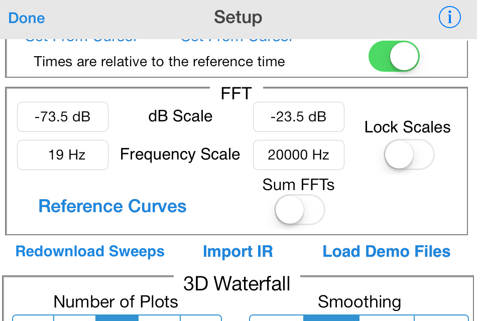
Here is the settings page for the FFT parameters. Note that the Reference Curves option is also available for this plot.
You can also lock the FFT graph scales and manually set the graph scale range from this screen.
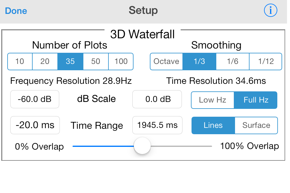
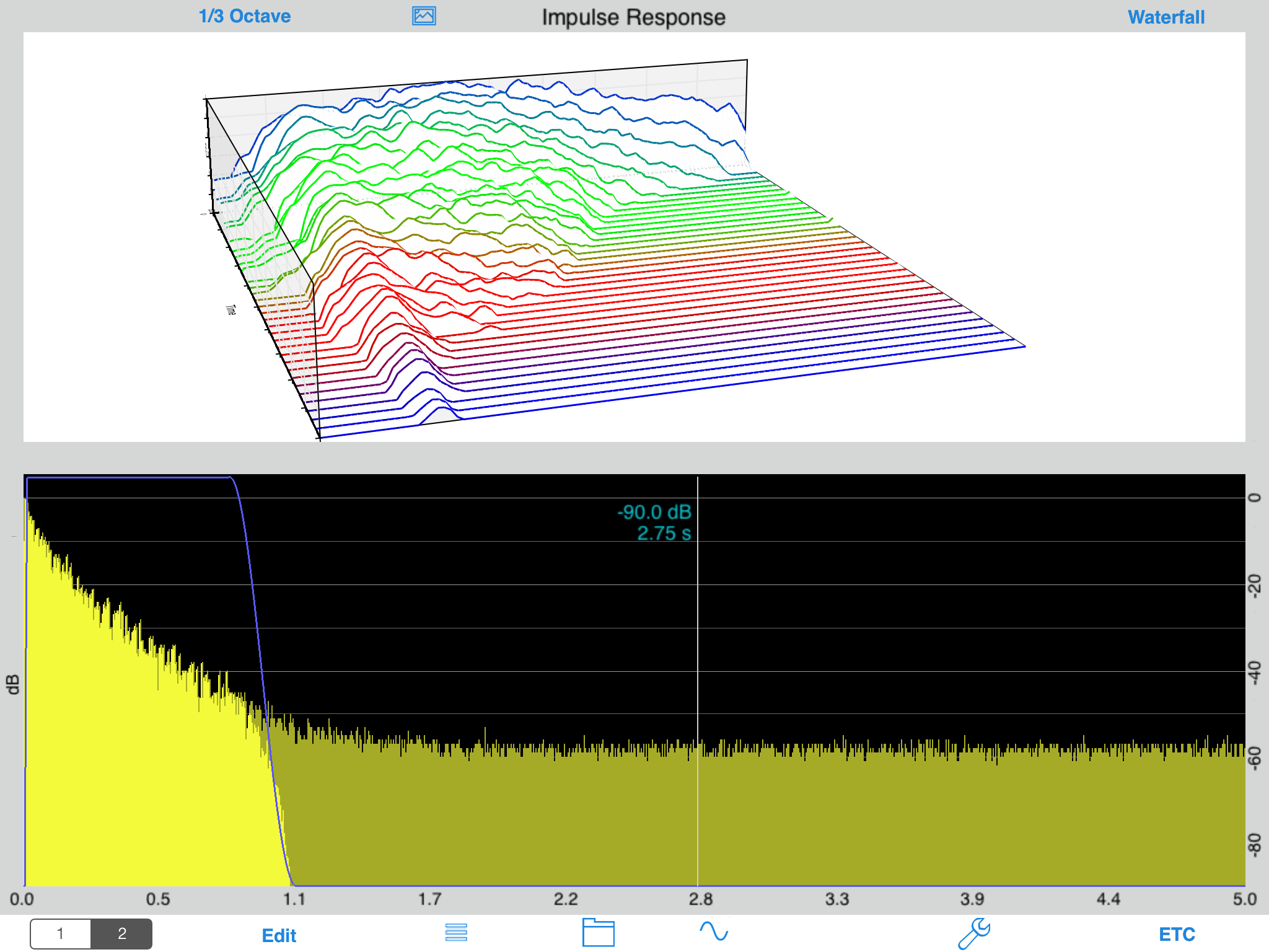
Waterfall Plots
A 3D waterfall plot that shows the decay of the sound spectrum by frequency over time may be shown. You can select between a plot of lines, or a solid surface. You can also select a full frequency plot, or just see the low frequencies.
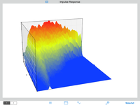
Waterfall plots are created by computing a number of individual FFTs, often called slices, each covering a small portion of the IR. The time range for the slices and the number of plots (slices) control the frequency and time resolution of the graph. You can also set the frequency smoothing for the plots, and the overlap, which will smooth the plots in time.
Here is the setup screen for the waterfall plots.
Summary Page
We have a summary page that shows a set of basic measurements:
T30/EDT/C50/C80 Mid Values – This is the average value for the Reverberation time, and Clarity in the measured room taken at the 500 Hz and 1 kHz Octave Bands.
S/N Broadband – The overall signal-to-noise ratio, expressed in dB of the measured IR.
Bass Ratio – The metric that correlates to the “warmth” of a room. It is calculated by adding the T30 values for the 125 Hz and 250 Hz octave-bands and dividing them by the sum of the T30 values for the 500 Hz and 1 kHz octave bands.
Impulse Response on iPad
iPad is an excellent platform for Impulse Response. Since we have more screen real estate, we allow splitting the screen into two graphs, so you can see two different plots at the same time. This is great for things like windowing, where you can adjust the window using the ETC plot and instantly see the results on the FFT plot.
Or, see the ETC and waterfall plots at the same time.
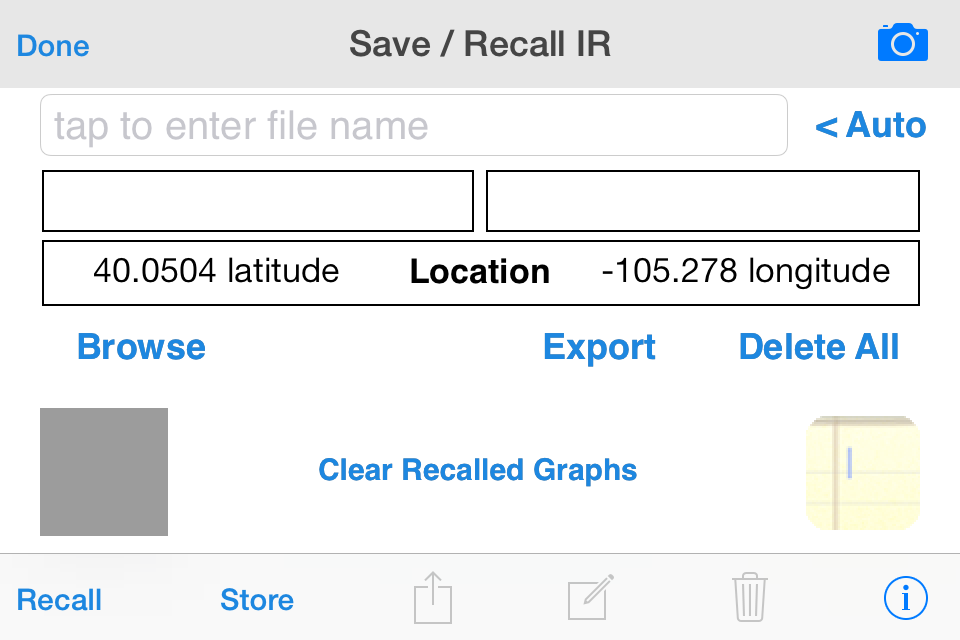
Saving Results
You can save an unlimited number of results on the device. For each IR, the raw audio file is saved, along with the processed IR. Also, a tab-delimited text file is saved that you can bring into any spreadsheet program.
You can enter your own text description, and the date/time and IR length are also stored with the data. You can even take a photo and store it with the IR. Se our Save / Recall page for more information.
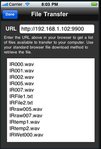
Uploading IR Data to Your Computer
The “wet” recorded IR, the result of the deconvolution, and a tab-delimited file of the final calculations can be uploaded to a PC or Mac. The IR can be used a source file for other programs. The tab-separated file is suitable for loading into Excel or any other typical editor.
Obtaining the Test Signals
Click this link to go to the page that has our IR chirp test signals. They are archived in a .zip file. The files include a 3.5s chirp 7s chirp and a 14s chirp Each chirp starts with a sync pulse 1 second after the file starts, 5 seconds of silence, the chirp, and another 5 seconds of silence. When you are recording the chirp, make sure that start recording first, then start the chirp file playing, and let the entire file including the ending sync pulse play before stopping the recording.
There are two versions of the sync files. Use the “syncxxx10.wav” if you need to use the 10-second expected maximum decay, otherwise use the “syncxxx.wav” files.